This article is about a project I did at the ISP at the University of Stuttgart. The second part is examining the transferability of our framework to other objects. We choose solar panel detection as such an other class, as there is a concrete demand to evaluate the development stages of renewable energies. Secondly solar panels exhibit a homogenous structure and are clearly visible and seperable, so an easy candidate for inference. In this case the goal is not to achieve the best inference results, but to test the transferability of our network.

Solar Detection

We can conceptually separate two cases of solar panels: Rooftop PV and Solar Parks. (For our case we do not distinguish between PV and Solar.) Since there is no data to efficiently segment the cases early in the predictions we need to make a model that covers both of these areas.

Using publically available training data

Since we already have the training and inference logic from the TreeDetection, we mainly lack datasets to train a new model. Here we use 4 major datasets and adapt their labeling to COCO-Format to train with them, the datasets are:

• MultiRes Dataset by Hou et al. available at Zenodo and the corresponding peer reviewed article in Copernicus.
• Crowdsource Dataset by Kasmi et al. available at Zenodo and the corresponding peer reviewed article in nature.
• SolarDK Dataset by Khomiakov et al. available at the OSF-Storgae website https://osf.io/aj539/ and their paper available at Arxiv. “OSFstorage Dataset”
• Germany Dataset by Clark et Pacifici with images available here by Maxar and annotations in a figshare here. The corresponding peer reviewed article in Nature.

These Datasets vary in different qualities and instances there are roof-pv, water-pv, and ground-mounted-pv. Together with a bit of filtering we have 22.407 images with 71043 training instances and 8622 test instances.

Evaluating the training we can see the precision and receive the results as:

applying inference to the trained model we get the following samples:

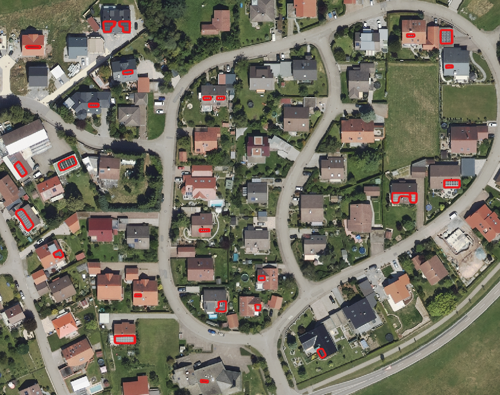
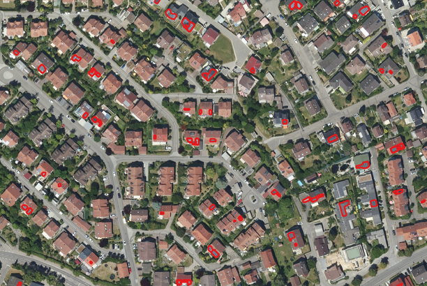
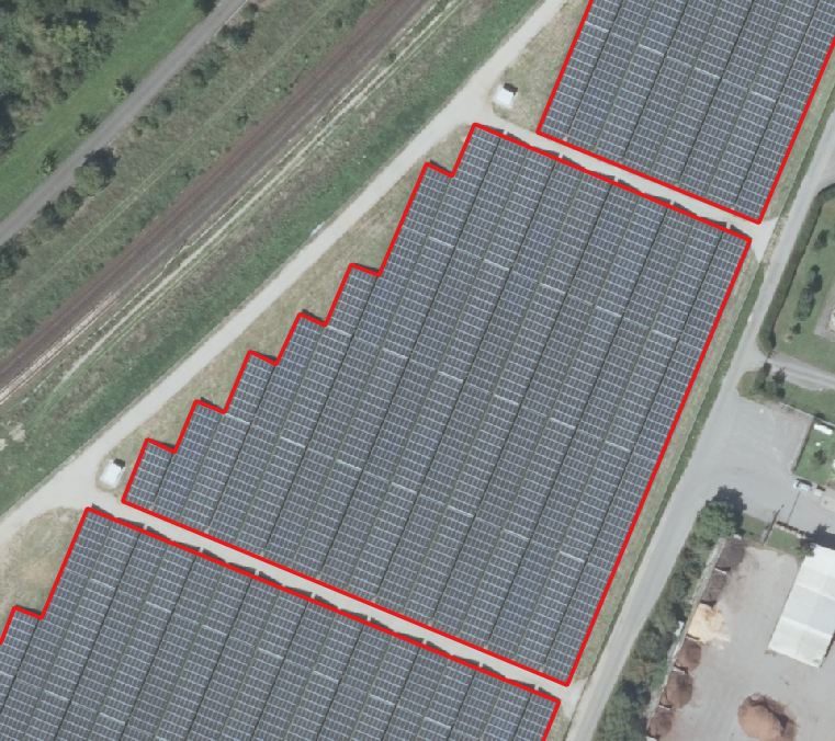
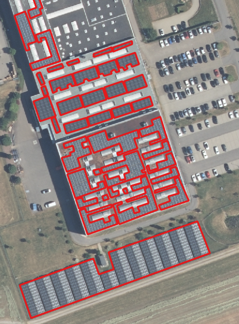
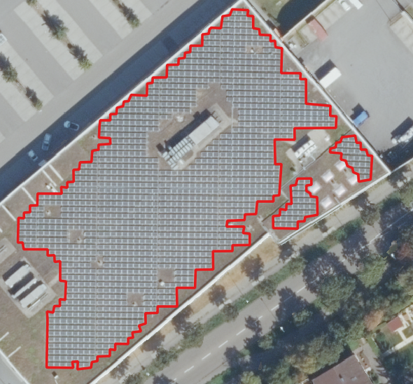
Samples of urban predictions of the model trained with only public informations.

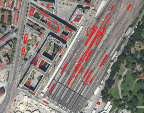
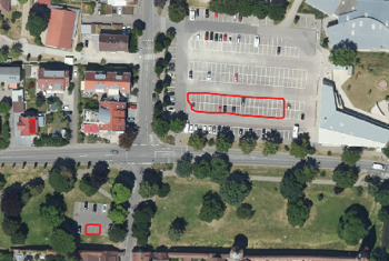
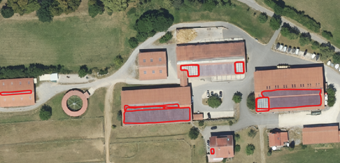
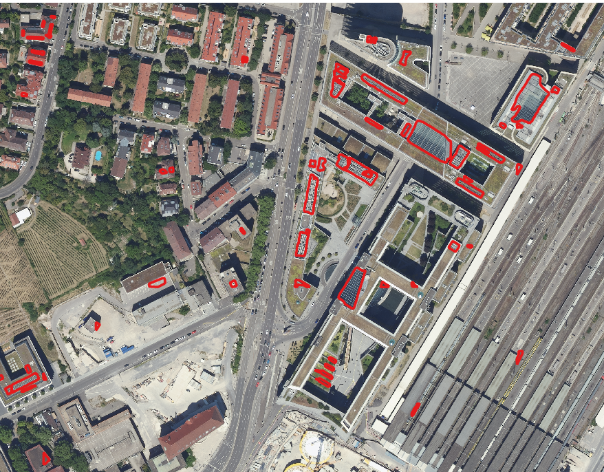
Samples of different kind of wrong predictions, such as in the first image: railway lines with similar rectangular patterns and roof lights, secondly from parking spaces and in the third image a hall with roof windows as well as solar panels (here it is even hard for humans to tell both apart).

So we can see the Precision is okay, but on a landwide scale there are several problems, especially since, many complicated structures especially in big cities are present in the real life inference data, that are not represented adequately in the training data. This leads to high confidence false positives. In order to mitigate this we have to further annotate real data.

Finetuning with our own data sets

We sampled different images as 1x1 km tiles using the OpenStreetMap Data with parameters as follows:

solar_tags = {
    "plant:source": "solar",
    "plant:method": "photovoltaic",
    "generator:source": "solar",
    "generator:method": "photovoltaic",
    "generator:type": "solar_photovoltaic_panel"
}
place_name = "Baden-Württemberg, Deutschland"

So we firstly extract everything with one of the tags and then we assign them to the special Tiles, this is because the annotations are very crude, some use single panels, some use the property lines or visual segmentations. Then we sample from these Tiles in 70 % single panels such as rooftop PV or single PV panels and 30 % from solar parks.

Then we manually annotate each tile, resulting in 26.398 geometries and an average of 126.91 geometries of tiles. You can see the distribution of panels below:

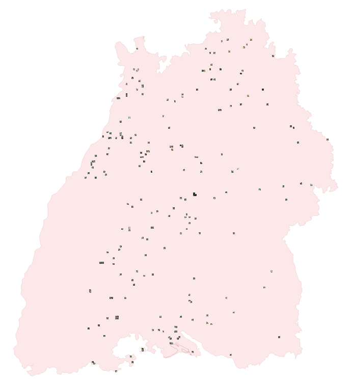
In order to efficiently capture solar parks with large panels we have a subtiling size of 50m and 70m buffer in each direction, this helps us to generate huge overlaps that can later be easily filtered and merged. We can then train/finetune the models using TensorFlow. We can see these precision curves:

	AP [50:95]	AP50
Bounding Boxes
Segmentation

These evaluations are notably worse than in pretraining, this is not because the models gets worse, but because our data is a lot more fine grained and complicated, more similar to real life conditions.

Adding features to enrich the data

Again, as in TreeDetection, we enrich each prediction with a lot of data, that allows for efficient filtering of wrong classifications and analysis of the predicted data:

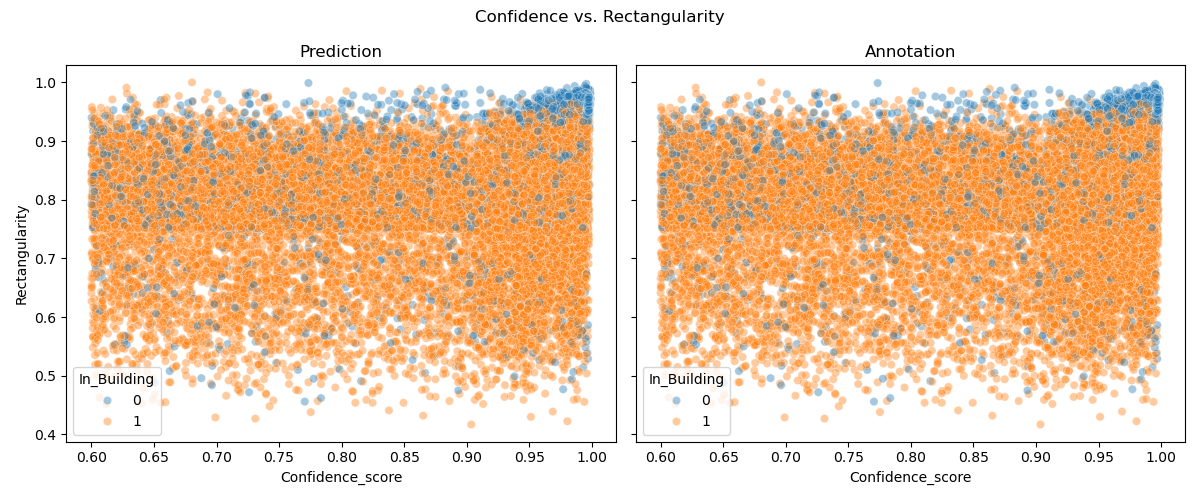
• Confidence Score As in every neural network each instance is predicted within a given certainty
• Centroid The geometric centroid of the shape.
• Height The height of the solar panels at the centroid.
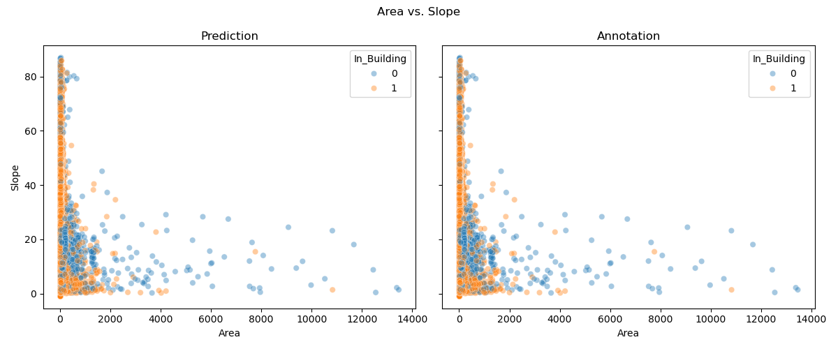
• Area The area of the polygon in square meters. This is meant as the area seen from above, note that in the case of movable panels, this area changes with the slope.
• True Area The total area of the solar panels corrected for the slope.
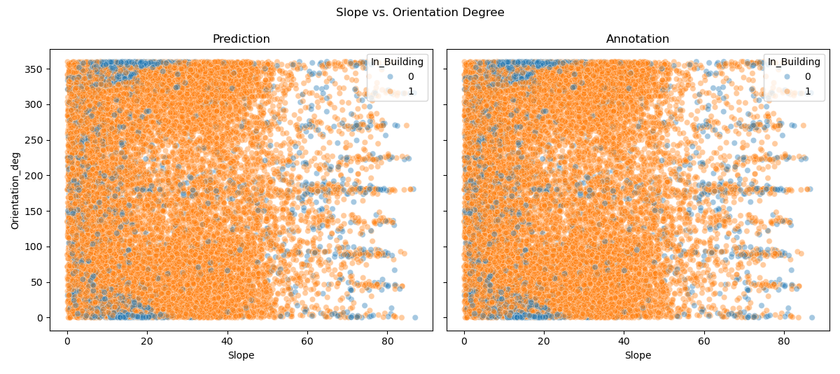
• Slope The slope of the panel.
• In_Building If a shape of buildings is provided this determines if the Solar panel is within a building, so rooftop solar or outside of a building, so ground-mounted solar, most likely a solar park.
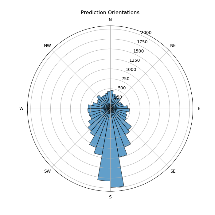
• Orientation_deg and Orientation_label the principal direction the panel is leaned towards to, determined by the gradient and a label (‘N’,’S’,…)
• Rectangularity and Shape_complexity Since most solar panels are rectangular, these two parameters measure how complex this shape is based on convexity and fitting a bounding box. This allows for better filtering later on.
• Containment Variables As in Trees hierachic Predictions have to be carefully sorted, for this the same containment variables are used, but the logic is different.
• AvgRGB An approximation of the color of the predicted instance, based on the centroids’s color.

Obviously if several panels are recognized together as one prediction, orientation and slope parameters become harder to estimate, we have accounted for this in the code, generally a high-res height raster is useful to mitigate errors.

Unfortunately, again the hierachic recognition is one of the main problems to consider in this case, since here again we have a lot of instances, that are clearly separable in some cases and less in others. So for instance in solar parks, the panels are sometimes spread out to avoid shadows, sometimes they are close by, when space is costly and sometimes there is no gap between them. The same holds for rooftop solar on large buildings.

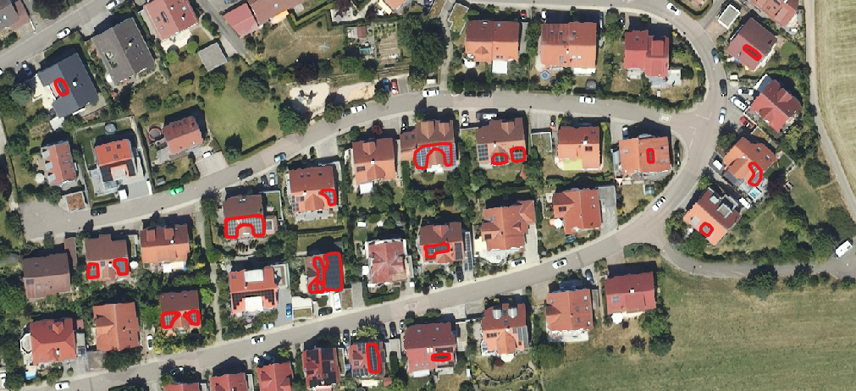
Some examples of different distances in the annotations are:

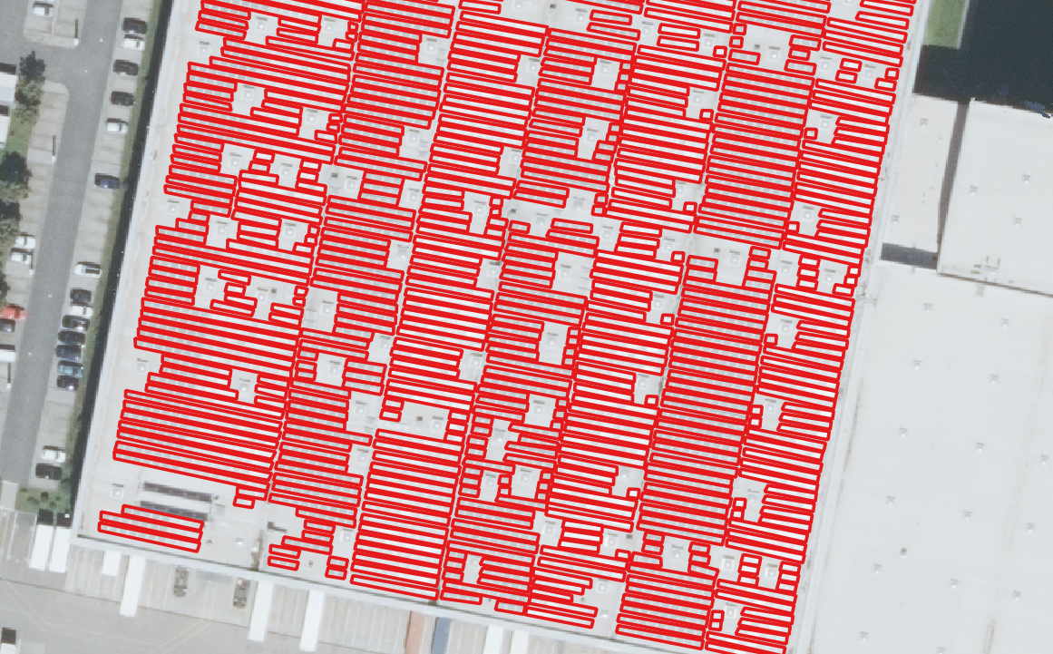
Samples of different different annotations in the training data with complicated file annotations.

This is fixed with our selection logic, together with other problems, such as detection of containers and cars that are visually very similar, but differ in environment, and small carports that are often detected. The postprocessing steps filter as follows:

1. Eliminate based on height and area thresholds.
2. Eliminate duplicates similar to the tree logic, but with more precedence to rectangular shapes for small area polygons.
3. Eliminate polygons based on rectangularity and shape complexit together with area and building information.
4. Eliminate based on height and slope information.
5. Eliminate based on containment.

By frequently combining building and area information we ensure a robust inference of both main groups, solar parks as well as rooftop pv.

We can compare the properties of predicted and annotated Geometries, to gain insight in the ways of our panels and get a high level overview:

Results

Since we do not provide an explicit test split in the dataset we only provide qualititative results as well as insights in the properties. In general we can see that the predictions on rooftop PV are qualitatively very accurate, the recall is high, but sometimes there are still some wrong predictions.

Image Samples

We have a few several different samples as a short showcase, you are always encouraged to make your own to try it!

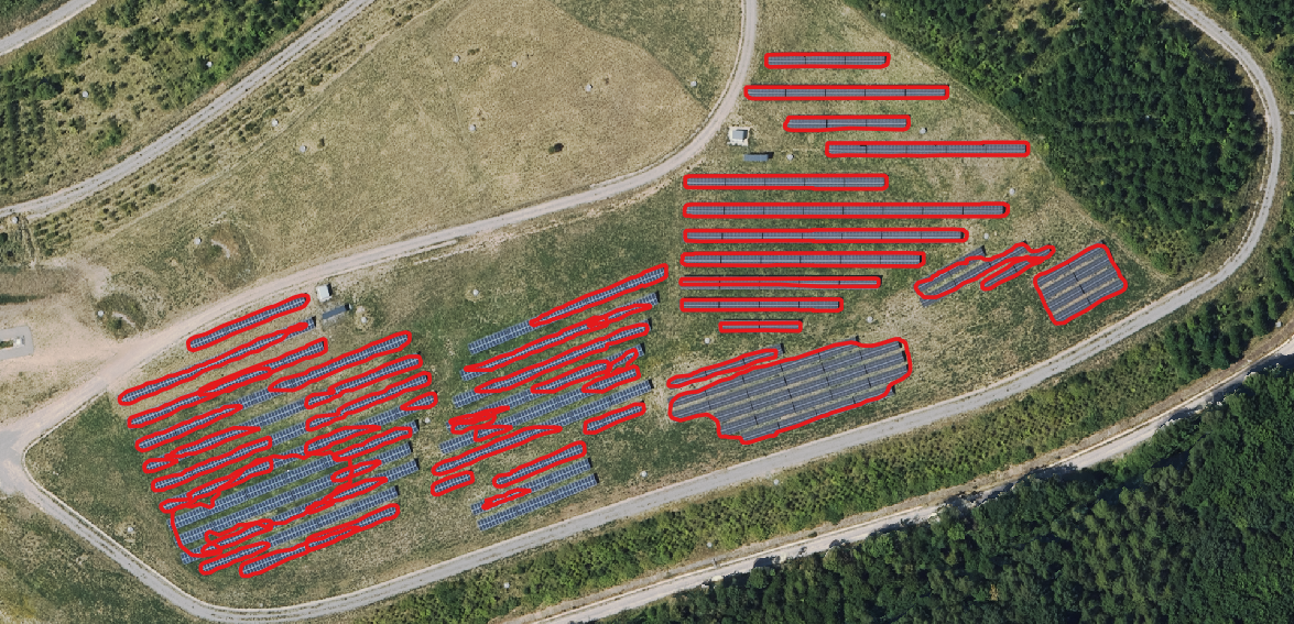
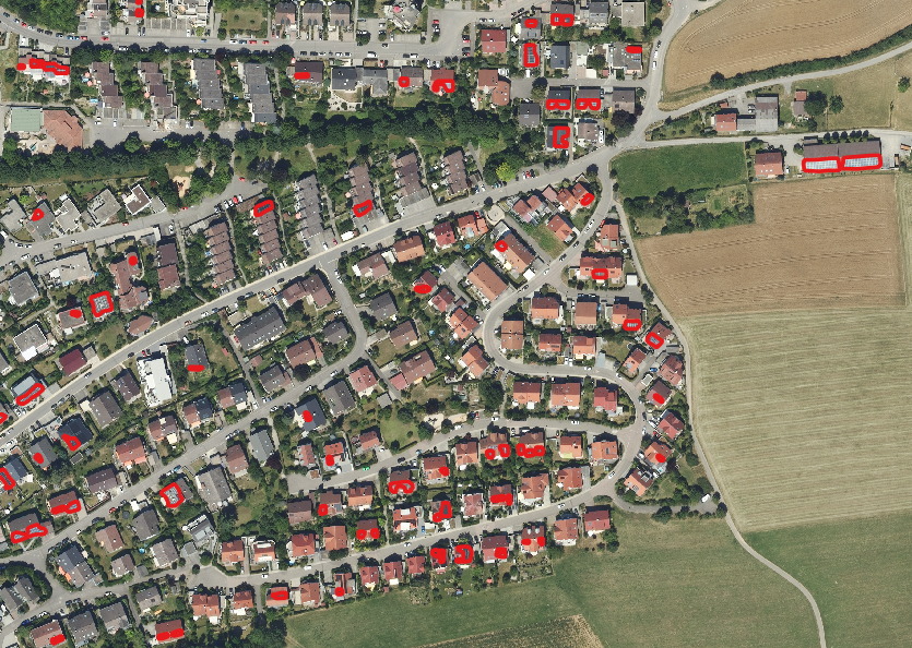
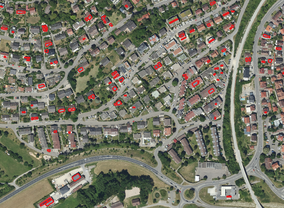
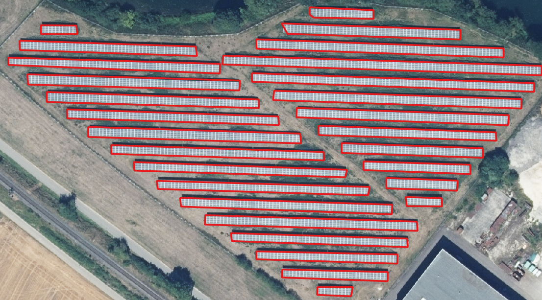
The predictions capture the majority of solar panel structures across different environments, from rural solar farms to dense urban and suburban rooftops. In the solar farm, the model delineates panel rows well but tends to fragment continuous structures into multiple smaller polygons. In urban and suburban areas, most rooftop panels are detected, yet there are occasional false positives and missing detections, especially on smaller or shaded installations.

Weaknesses & Limitations

The main weaknesses of the predictions are inconsistent segmentation quality and sensitivity to context. Large, continuous panel areas are often broken into many smaller polygons, while in urban and suburban settings, small or partially shaded panels are sometimes missed entirely. False positives also occur on dark roof patches or non-panel structures, highlighting limited robustness to visual variability. These issues suggest the model struggles with both fine-grained precision and generalization across different environments.