This article is part of a larger series of introductory AI tutorials for non-techies, written in German and auto-translated.

For a change, this is a mathematical article that deals with the behavior of probability distributions and their laws in higher dimensions. We use these rules in the second step to gain an intuition for certain properties of systems in machine learning. Many statements in this chapter are not fully derived or mathematically verified—this is intentional. The aim is to provide insight into the geometric interpretation of various phenomena without delving into complicated formalisms.

1. Motivation

A “data dimension” is not the same as a spatial dimension in the physical sense. We understand a dimension to be any degree of freedom—i.e., any component of a vector space that can be changed independently. More precisely, it is the number of variables or characteristics that make up a data point. We speak of high dimensionality when the number of dimensions is large in relation to the number of data points or when we generally have many characteristics (often double digits or more). Since we are particularly interested in the mathematical laws that arise when the dimension increases, we do not analyze specific values, but rather consider the behavior in the limiting case of very high dimensionalities.

Why are we interested in this behavior?

When processing complex data, we rarely have just a single feature, but many. It often even makes sense to artificially increase the dimensionality in order to better capture interactions between features and extract patterns. Deep learning further amplifies this effect: each neuron can be interpreted either as a transformation of the original vector space or as the generation of a new feature in the latent space. In this article, we focus primarily on the latter view: neurons as feature generators. Since stochastic methods and probability distributions play a central role in training, the question arises: How can we actually imagine what a model “sees” and ‘learns’ in so many dimensions? The next chapter is therefore devoted to a series of counterintuitive phenomena in high dimensions. I will try to make the derivation as accessible as possible without using difficult equations – but in a few places there will necessarily be a “trust me, bro” moment. If you like, you can of course question these points critically and think further for yourself. The aim of this article is to give you a better understanding of the basics of high dimensions after reading it, so that mechanisms such as diffusion, adversarial networks (GANs), randomized projections, and attention can be better understood.

This article is largely based on a lecture by Dirk Pflüger, who vividly illustrated the topic as follows: Why is soccer in 10 dimensions not fun? One might ask: Why do most shots miss the goal? And why does it matter who I pass to – after all, everyone is standing on the sideline anyway? A question more closely related to machine learning is: Why do we keep adding small amounts of noise to diffusion models instead of adding it all at once? Or why do generative adversarial networks (GANs) quickly become unstable, and what problems does this cause for us?

2. Interesting phenomena in high dimensions

We assume some basic statistical concepts such as variables, probability spaces, expected value, variance, Landau notation, independence, normal distributions, and uniform distributions so that we do not have to define everything here. The variables d and n always represent the dimensionality of the space. Other fundamentals include the law of large numbers, which states that if we average many independent random values with the same expected value, then this average will approach the actual expected value with increasing certainty as the number grows, and Chebyshev’s inequality, which guarantees that the probability of large deviations from the expected value quickly becomes small by controlling the distance of a random variable from its mean by its variance.

We assume some basic knowledge of statistics—such as variables, probability spaces, expected value, variance, Landau notation, independence, normal distributions, and uniform distributions—so that we do not have to define everything here. The variables d and n always represent the dimensionality of the space. Other basic concepts include the law of large numbers, which states that when averaging many independent random values with the same expected value, the average will increasingly closely approximate the actual expected value as the number of values increases, and Chebyshev’s inequality, which guarantees that the probability of large deviations from the expected value quickly becomes small by controlling the distance of a random variable from its mean by its variance.

Features in high dimensions (norm concentration)

Let us consider where the mass of a high-dimensional variable $X = (X_1, X_2, … ,X_n)$ is located, where the individual features $X_i$ are independent and have the same expected value and equal and finite variance. In neural networks and similar methods, it is common to normalize the features beforehand; independence is a method often used to simplify the problem. Considering the norm, a new stochastic variable $X’ = \sqrt(X_1^2+X_2^3 + … + X_n^2)$ for which $\mid \mid X\mid \mid _2 = X’$. Now we can determine the expected value of $X$:

$E(\mid \mid X\mid \mid 2^2) = \Sigma{i=0}^n E(X_i^2) = n\sigma ^2 $

To do this, we can use the variance for the mean of the squares of the individual features, since the value converges to this variance in high dimensions (law of large numbers):

$ \frac{1}{n} \Sigma_{i=0}^n X_i^2 \rightarrow \sigma^2\ $ for $ n \rightarrow \infty$

Then, the expected value of $\mid \mid X\mid \mid $ can be used in this equation:

$ \frac{\mid \mid X\mid \mid 2^2}{n} = \frac{1}{n}\Sigma{i=0}^n X_i^2 \approx \sigma^2\ \ $

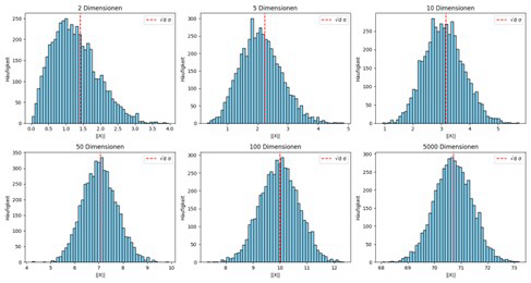
In high dimensions, this results in a concentration of the norm around $\sqrt{n}$:

$ \mid \mid X\mid \mid _2 \approx \sqrt{n} \sigma \ \ $ for large $n$

Furthermore, the Law of Large Numbers shows that the variance decreases as $d$ increases. This derivation is discussed in detail in the next chapter and is skipped here.

What does that mean geometrically? Geometrically, it means that the mass of the distribution lies in a very thin spherical shell around the center with radius d. It also means that in high dimensions, the magnitude of values is almost irrelevant and only the angles and correlations between vectors contain information.

What does this mean in terms of application? This means that we can stabilize the variables by mapping individual features to a normal distribution. Example:

• BatchNorm and LayerNorm automatically normalize the vectors to a fixed length, thereby preventing exploding gradients and diminishing returns.
• The typical scaling in attention mechanisms by $\frac{1}{\sqrt{n}}$ results from this in order to return to the thin spherical shell in which we want to calculate.
• In diffusion models, these high-dimensional noise vectors serve to stabilize the norm so that we can create a traceable path through this spherical shell.

What does this look like experimentally?

We can estimate this standard concentration as follows, for example:

import numpy as np
import matplotlib.pyplot as plt
# ------------------------------
# Parameter
# ------------------------------
dimensions = [2, 5, 10, 50, 100, 5000] # Different Dimensions
n_samples = 5000 # Vectors per dimensions
sigma = 1.0 # Standard deviation 
distribution = 'uniform' # distributions: 'uniform' or 'normal'
# ------------------------------
# Simulation of the norms
# ------------------------------
norms_dict = {}
for d in dimensions:
 # X = n_samples x d Matrix, Features i.i.d. N(0, sigma^2)
 X = np.random.normal(loc=0, scale=sigma, size=(n_samples, d))

 # COmpute the norms
 norms = np.linalg.norm(X, axis=1)

 # Safe in dict
 norms_dict[d] = norms
# ------------------------------
# Plot: Histograms of the Norms
# ------------------------------
plt.figure(figsize=(15, 8))
for i, d in enumerate(dimensions):
 plt.subplot(2, 3, i+1)
 plt.hist(norms_dict[d], bins=50, color='skyblue', edgecolor='k')
 plt.title(f'{d} Dimensions')
 plt.axvline(np.sqrt(d)*sigma, color='r', linestyle='--', label='d ')
 plt.xlabel('||X||')
 plt.ylabel('Frequency')
 plt.legend()
plt.tight_layout()
plt.show()

The result of the standard concentration is as follows:

Distances in high dimensions (measure concentration)

We consider two random points that originate from the same distribution. To do this, we define the vectors as $X = (X_1, X_2, … ,X_n)$ and $Y=(Y_1, Y_2, … , Y_n)$, where the individual components are independent random variables with finite variance. The Euclidean distance between these points can be described as

$\mid \mid X-Y\mid \mid _2 = \sqrt{((X_1^2 + … + X_n^2) - (Y_1^2 + … + Y_n^2))}$

For large $n$, the expected values of each individual variable can be used. Thanks to the Law of Large Numbers, we know that the mean values of the random variables are almost exactly equal to their expected value and variance:

$E(X) = \frac{1}{n} \Sigma_{i=0}^n X_i = \frac{1}{n} \Sigma_{i=0}^n E(X_i)$ and $Var(X)=\frac{1}{n^2} \Sigma_{i=0}^n Var(X_i)$

Thus, we can determine (analogously for $Y$):

$E(X) = \mu$ and $Var(X) = \frac{\sigma^2}{n}$

Chebyshev’s inequality provides an upper bound for the dispersion, so we can see that as $n$ increases, the random values become increasingly dense around the mean. This results in:

$P(\mid X-\mu \mid > \epsilon) \leq \frac{Var(X)} {\epsilon^2} = \frac{\sigma^2}{n \cdot \epsilon^2} \approx 0 $ with $n \rightarrow \infty$

Applied to the norm $\mid \mid X-Y\mid \mid $, this means that this distance is highly likely to be approximately $E(X-Y) = \sqrt{\Sigma_{i=0}^n(X_i-Y_i)^2} = \sqrt{n \cdot E(X-Y)^2}$.

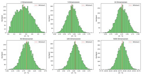
What does this mean geometrically? The Euclidean distance between two data points is therefore strongly concentrated around the expected value. Practically all distances hardly differ from each other. This can be represented geometrically: Choose a distribution, for example an even distribution on $[0,1]$, and apply it to different dimensions:

• $1$ dimension $\rightarrow$ line
• $2$ dimensions $\rightarrow$ square
• $3$ dimensions $\rightarrow$ cube
• $n>3d\rightarrow$ simulation necessary

Always select two points, calculate the distance, and record it in a histogram. In theory, the variance of the distance decreases with increasing dimension – the rate of decrease is approximately $O(\sqrt{n})$.

What does this mean in terms of application? Distances between individual data points are hardly distinguishable in high dimensions and are therefore problematic as a metric. In contrast, however, the distance between samples from different clusters is robust. Examples:

• Nearest neighbor search does not work reliably.
• High separability in high-dimensional spaces (e.g., double descent phenomenon).
• Different samples from normally distributed sources have a distance of approximately $\sqrt{2 \cdot n}$, which can be used by separating Gaussians, for example.

What does this look like experimentally?

We can simulate the distance concentration as follows:

# ------------------------------
# Simulation
# ------------------------------
distances_dict = {}

for d in dimensions:
    distances = []
    
    for _ in range(n_samples):
        if distribution == 'uniform':
            X = np.random.uniform(0, 1, d)
            Y = np.random.uniform(0, 1, d)
        elif distribution == 'normal':
            X = np.random.normal(0, 1, d)
            Y = np.random.normal(0, 1, d)
        else:
            raise ValueError("Distribution not available.")
        
        # euclidian distance
        dist = np.linalg.norm(X - Y)
        distances.append(dist)
    
    distances_dict[d] = distances

# ------------------------------
# Plot: Histograms of the dimensions
# ------------------------------
plt.figure(figsize=(15, 8))

for i, d in enumerate(dimensions):
    plt.subplot(2, 3, i+1)
    plt.hist(distances_dict[d], bins=50, color='lightgreen', edgecolor='k')
    plt.title(f'{d} Dimensions')
    plt.xlabel('||X - Y||')
    plt.ylabel('Frequency')
    plt.axvline(np.mean(distances_dict[d]), color='r', linestyle='--', label='Average')
    plt.legend()

plt.tight_layout()
plt.show()

The result visualizes distance concentration in different dimensions and shows how distances in high-dimensional spaces become nearly equal:

Angles in high dimensions (near orthogonality)

The basis for this chapter is $a^2 + b^2 = c^2$ (Pythagorean theorem). A high-dimensional variant of this theorem is given in the equation: $H=\mid \mid X \mid \mid_2 = \sqrt{\Sigma_{i=0}^n X_i^2}$

The proof for this statement can be easily done by induction over the number of dimensions. As can be seen, the hypotenuse length is equal to the $L2$ norm.

In addition, we now consider features that are normally distributed. The idea is: We construct a triangle between two points and the origin and consider the angles of the triangle using the Pythagorean theorem.

Derivation The use of normally distributed features leads to a chi-square distributed multidimensional variable $\mid \mid X\mid \mid ^2$. The expected value of this norm is very reliably $\sqrt{n}$, as already demonstrated in Section 2.1. This follows from the norm concentration of vectors with independent features.

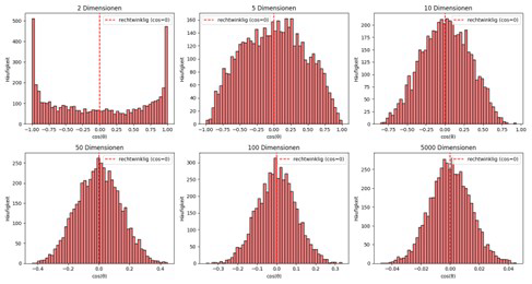
The distance between the two points—i.e., the hypotenuse of the triangle—can be squared as $E(\mid \mid X-Y\mid \mid ^2)$ using the normal distribution of the individual variables $X$ and $Y$. Since $X$ and $Y$ consist of components with variance $1$ and expected value $0$, inserting the result from section 2.2 (distance concentration) yields a value of $2n$. This means that we have a high probability of a distance of 2d for the hypotenuse and a distance of d for the legs. According to Pythagoras’ theorem, this always corresponds to an almost right angle.

What does this mean geometrically? Points originating from approximately normally distributed features are almost always perpendicular to each other in high-dimensional spaces.

What does this mean in terms of application? In many machine learning algorithms, this near-orthogonality produces stable sampling of the high-dimensional space. An example of this is a step along an orthogonal path by adding d-dimensional noise, which leads to a new instance in the latent space (e.g., in diffusion or generative networks).

What does this look like experimentally?

We can simulate the angles as follows:

# ------------------------------
# Simulation
# ------------------------------
cos_angles_dict = {}

for d in dimensions:
    cos_angles = []
    
    for _ in range(n_samples):
        # Two Vectors X, Y with i.i.d. N(0,1) Components
        X = np.random.normal(0, 1, d)
        Y = np.random.normal(0, 1, d)
        
        # Cosine of the Angle X and Y
        cos_angle = np.dot(X, Y) / (np.linalg.norm(X) * np.linalg.norm(Y))
        cos_angles.append(cos_angle)
    
    cos_angles_dict[d] = cos_angles

# ------------------------------
# Plot: Histograms of the Angle cosine
# ------------------------------
plt.figure(figsize=(15, 8))

for i, d in enumerate(dimensions):
    plt.subplot(2, 3, i+1)
    plt.hist(cos_angles_dict[d], bins=50, color='lightcoral', edgecolor='k')
    plt.title(f'{d} Dimensions')
    plt.xlabel('cos(θ)')
    plt.ylabel('Frequency')
    plt.axvline(0, color='r', linestyle='--', label='angle (cos=0)')
    plt.legend()

plt.tight_layout()
plt.show()

The result can be visualized as follows:

Volume in high dimensions

In this chapter, we will examine how the volume of objects is distributed in higher-dimensional spaces and what statements we can make about these objects.

Special volume of a cube

Let us consider a high-dimensional cube $A$ and reduce it by a very small factor $\epsilon$. Comparing the volumes of both cubes shows that as soon as the cube is shrunk, the proportion of volume inside the cube rapidly approaches zero:

$\frac{Vol((1-\epsilon)A)} {Vol(A)} = (1-e)^n \leq e^{\epsilon \cdot n} \rightarrow 0$ with $n \rightarrow \infty$

In terms of application, this means that even with evenly distributed sampling, the volume within the object is not evenly distributed. Therefore, rule-based methods or grid structures must be used with caution in high dimensions.

Special volume of a sphere

The volume of a sphere in $d$ dimensions can be calculated using a closed formula, depending on the radius and dimension. Analogous to the cube, one can estimate how much volume lies within a thin layer that is created when the sphere is shrunk by $\epsilon$. A detailed derivation and proof of the closed formula can be found, for example, on Wikipedia. Example: With $\epsilon=\frac{1}{d}$, approximately $63\%$ of the volume is in the inner layer, which is $\frac{1}{d}$ away from the edge. It can also be seen that both the surface area and the volume – regardless of the radius – tend very strongly towards zero as the dimension increases.

3. Use cases

Enough theory, now let’s turn to practice.

Let’s recall what we know so far:

• Independent and evenly distributed features with finite variance generate feature vectors that move around a radius $O(1)$ or a multiple of $\sqrt{n}\sigma^2$ ; in normalized inputs, this means in a circular disc around $\sqrt{n}$.
• The distances between these features are almost identical.
• The angles between the features are almost orthogonal.
• Most objects have their volume very close to the surface, but are practically empty inside.
• Spheres tend strongly towards zero in both volume and surface area as the dimension increases.

What does the feature space of high, normally distributed variables look like? This is not easy to answer, as we cannot imagine the dimensions. However, we know that the features lie on a circular disc around the origin and are arranged on this circular disc in a quasi-orthogonal grid.

Diffusion models

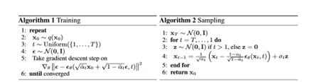
Let us consider Denoising Diffusion Probabilistic Models (DDPMs), which were introduced by Ho et al. in 2020. These work in a two-step process:

Training: During training, we always add a normalized vector with a length of √d to the previous point. This allows us to move on the circular disc and on the orthogonal grid, away from the instances, in a stable path with a constant “length” (depending on the time parameter $t$). In other words, we learn the relative direction to a semantic region, not the absolute position. By adding the normalized vector, the gradient is updated extremely stably, which allows larger, more semantic fields to be learned more precisely than with classic gradient descent. We thus learn smooth curves that lead to different targets instead of just a general average (mode collapse).

The forward pass can be used with a mathematical model to obtain a specific sampling point and time $t$:

$q(x_t \mid x_0) = N(\sqrt{\alpha_t}x_0, (1-\alpha_t) I)$ with $\alpha$ as the temperature parameter.

Important here is the isotropy in the variance, which favors a smooth probability distribution on the paths to $x_0$.

Sampling: During the sampling process, normalized noise helps us in a hierarchical procedure. The isotropic noise $z$ ensures norm stability and orthogonality. The iterative application of this noise ensures that we do not simply move to the learned center point, but rather move back and forth on similar smooth curves, thus reaching a “correct” point. Both $x$ and $z$ remain normally distributed; thus, we do not leave the circular disc on which we are calculating and on which the majority of all valid instances lie. Theoretically, the isotropic noise does not directly change the target direction, but it helps to query the model more specifically for semantic regions instead of simply following the learned path.

More advanced topics such as process-oriented interpretation of diffusion, DDIMs, or class-free diffusion are not explained, as this would go beyond the scope of this article. The blog Sander.ai is a good resource for further information on this topic.

Transformers

Within Transformers, high-dimensional properties play a particularly important role in calculating attention. Scaling using $\sqrt{n}$ (the number of dimensions) results from norm concentration and enables stable training, as the results of the scalar products of query and key vectors lie back on the circular disc of the samples. The scalar product between $q$ and $k$ remains stable only because the vectors in high-dimensional space are almost orthogonal to each other. Without this near-orthogonality, training would collapse from the outset. In addition, separability in high-dimensional spaces—a consequence of orthogonality and norm concentration—ensures that any normally distributed initialization of the weight matrices of $q$ already provides a good starting point for enabling meaningful separations. This is closely related to the principle of random projections.

Calculation of the attention score based on query and key: $score(q, k) = \frac{q \cdot k}{\sqrt{n}}$

Further simple explanations

Semantic embeddings Norm concentration makes it clear that distances in high dimensions are often no longer meaningful for capturing differences between latent representations. The near-orthogonality of independent vectors also implies that non-orthogonal vectors must be dependent on each other. Therefore, cosine similarity is a suitable measure for the relationship between vectors.

LayerNorm & BatchNorm Performing normalization on each layer is often difficult, which is why LayerNorm and BatchNorm are used. They ensure that the instances are brought back to the “circle disc” of the feature vectors and that large deviations are stabilized.

Glorot and He initializations for layers To accelerate training from the ground up, the layer weights are initialized with Xavier (Glorot) or He (Kaiming) initializations. This ensures that a normalized vector with length $n$ remains approximately normalized after the transformation.

Clustering in high dimensions Algorithms such as k-Nearest Neighbor or DBSCAN, which are commonly used to identify cluster structures, hardly work in high dimensions due to the concentration of measures. The distances between the points become almost equal, making it very difficult to distinguish between clusters.

4. Manifold Hypothesis - How can I resolve these issues?

In this article, we have examined how high-dimensional data points can be interpreted and what properties arise in high-dimensional stochastics. However, depending on the application, these properties can also be disadvantageous: Degeneration of distances, lengths, and angles is not always desirable. A key approach to circumventing these problems is to reduce the dimensionality to a few dimensions in which many classic statistical tools can be applied meaningfully again. This is precisely the core of the manifold hypothesis.

Manifold hypothesis: The manifold hypothesis states that real data in a high-dimensional space is located only on a thin surface (manifold) on which the data points are completely explainable.

Example: An image of an object with $64×64$ RGB pixels theoretically has $12,288$ dimensions. However, if some pixels are already set, the space of possible values for the remaining pixels is reduced, resulting in a loss of degrees of freedom. Conceptually, this can be imagined as a 2D surface in 3D space: All realistic instances of the object lie on this surface. It would be desirable to approximate this intrinsic structure of the data. In such a low-dimensional space, each variable becomes more significant and represents a more abstract representation of the instance. These low-dimensional, latent representations can be generated in various ways: Classic methods such as random projections, principal component analysis (PCA), linear discriminant analysis (LDA); nonlinear methods such as t-SNE or UMAP; and advanced methods such as autoencoder-based embedding models. These approaches help to capture the intrinsic structure of the data while reducing the problems of high-dimensional stochastics.

5. Conclusion – What have we learned?

In this article, we have examined the behavior of probability distributions in high-dimensional spaces and investigated the geometric laws that result from them. Many of the phenomena seem counterintuitive at first: norms concentrate, distances hardly differ, vectors are almost orthogonal, and volume shifts almost completely to the surface of objects. However, these properties provide valuable practical insights into how certain operations in machine learning can be interpreted. We have seen examples where the behavior of algorithms is directly influenced by properties of high-dimensional stochastics. In the last section, we took a brief detour to discuss the manifold hypothesis, which states that our data lies in smooth subspaces of the actual variable space. The important thing here is not to remember all the derivations in detail, but to gain a holistic view of how operators, data, and dimensions can be interpreted geometrically. Many of our intuitive rules from classical, low-dimensional space no longer apply here—and it is precisely this counterintuitiveness that shapes the behavior of algorithms in high-dimensional spaces.